From Target to Operator: Mixture, Selection, and Synthesis

Designing Training Data for Language Models · Part 3 of 3
When to optimize, what makes data good, and how to change it.
Advancement vs. Acceleration · What Makes Data Good? · From Target to Operator

Suppose we want a language model to perform better on a target—a domain, a task, or a set of capabilities—and can change the data it trains on. Which changes should we make?

One objective, three operators

A direct way to pose the problem is to choose a training distribution $q$ by evaluating the model $\theta^*(q)$ it produces on the target. Let $\mathcal Q$ be the family of training distributions available to us. This gives a bilevel objective:

\[\min_{q\in\mathcal Q} \mathcal L_{\mathrm{target}}\!\left(\theta^*(q)\right) \quad\text{s.t.}\quad \theta^*(q)\in\arg\min_\theta \mathbb E_{x\sim q}[\ell(x;\theta)].\]

The inner problem trains the model on $q$. The outer problem chooses that distribution to improve the trained model’s target performance.

The previous essay develops the motivation for this view. Here, we turn to the “how”: what changes can we make to the training data, and how can we find changes that move us toward that goal? The first concerns the data operator, and the second concerns the solver.

Three common operators are to adjust the proportions of data from different domains (mixture), choose examples or tokens from an existing pool (selection), or generate new training examples (synthesis).

Operator	Decision variable	What it can change	Its boundary
Mixture	Domain proportions	Exposure across predefined groups	Cannot distinguish examples inside a group
Selection	Example or token weights	Exposure within an existing pool	Cannot create a missing mode
Synthesis	Generator, prompt, or task specification	The examples available for training	Does not guarantee useful or correct data

Each operator defines a different feasible family $\mathcal Q$. Mixture and selection change exposure within existing data. If a useful behavior is present but rare, reallocating exposure may help. If the required training material is absent, we need to collect or generate it. Synthesis lets us change which examples are available, extending distribution design beyond reallocation.

Choosing an operator gives us a set of decisions—domain proportions, token masks, or generation choices. For a given operator, we still need to optimize its decision variables. The most literal approach is to propose a mixture, train a language model, evaluate it on the target, and repeat until the compute budget, or our patience, runs out. Trying every possible subset for selection is even less inviting. Can we optimize these data decisions without solving the training problem from scratch for every candidate?

From the bilevel objective to an allocation update

We first consider mixture and selection, where the decision is how to allocate training exposure within existing data. Let $w$ denote these allocation variables and $\mathcal W$ their feasible set. For mixture, $w_k$ is the sampling proportion of domain $k$; for selection, $w_p$ is the selection weight of candidate $p$. Their dimensions and constraints differ, but both induce a training distribution $q_w$.

Writing $\mathcal L_{\mathrm{train}}(\theta;w)=\mathbb E_{x\sim q_w}[\ell(x;\theta)]$, we can express the same bilevel objective in terms of $w$. We use $\theta^*(w)$ as shorthand for the model trained on $q_w$. Synthesis will require a different parameterization, which we return to below.

We use a penalty reformulation to turn the coupled bilevel problem into a single-level optimization problem. Let $V(w)=\min_\theta\mathcal L_{\mathrm{train}}(\theta;w)$ be the minimum training loss under allocation $w$. We penalize the excess training loss above this minimum:

\[H_\lambda(w,\theta) =\mathcal L_{\mathrm{target}}(\theta) +\lambda\left[ \mathcal L_{\mathrm{train}}(\theta;w)-V(w) \right], \qquad\lambda>0.\]

The target term encourages low target loss, while the penalty encourages the model to approximately satisfy the inner training constraint. This construction introduces two model roles: a proxy, trained to approximate the minimum in $V(w)$, and a reference, trained on target loss plus a weighted training loss. Their ideal optimization targets are:

\[\begin{aligned} &\theta_{\mathrm{proxy}}^*(w) \in\arg\min_\theta\mathcal L_{\mathrm{train}}(\theta;w),\\ &\theta_{\mathrm{ref}}^*(w) \in\arg\min_\theta\left[ \mathcal L_{\mathrm{target}}(\theta) +\lambda\mathcal L_{\mathrm{train}}(\theta;w) \right]. \end{aligned}\]

The algorithms coordinate updates of the two models and the allocation. The proxy parameters $\theta_{\mathrm{proxy}}$ take gradient steps on training loss, while the reference parameters $\theta_{\mathrm{ref}}$ take steps on target loss plus the weighted training loss. Both use a finite number of steps to approximate the minimization problems above.

For the allocation update, we hold $\theta_{\mathrm{proxy}}$ and $\theta_{\mathrm{ref}}$ fixed and use the proxy to approximate the inner minimum. We then differentiate the resulting loss contrast with respect to $w$:

\[\begin{aligned} &\partial_w\left\{\lambda\left[ \mathcal L_{\mathrm{train}}(\theta_{\mathrm{ref}};w) -\mathcal L_{\mathrm{train}}(\theta_{\mathrm{proxy}};w) \right]\right\}\\ &=\lambda\left[ \partial_w\mathcal L_{\mathrm{train}}(\theta_{\mathrm{ref}};w) -\partial_w\mathcal L_{\mathrm{train}}(\theta_{\mathrm{proxy}};w) \right]. \end{aligned}\]

For the specific mixture and selection formulations outlined in the next two sections, training loss is linear in $w$. The allocation update therefore reduces to the loss difference:

\[s_i= \mathcal L_{\mathrm{train}}^i(\theta_{\mathrm{proxy}}) -\mathcal L_{\mathrm{train}}^i(\theta_{\mathrm{ref}}).\]

Here $i$ indexes domains for mixture and tokens for selection. The allocation gradient estimate is proportional to $-s_i$, so descent favors larger $s_i$, subject to the operator’s constraints.

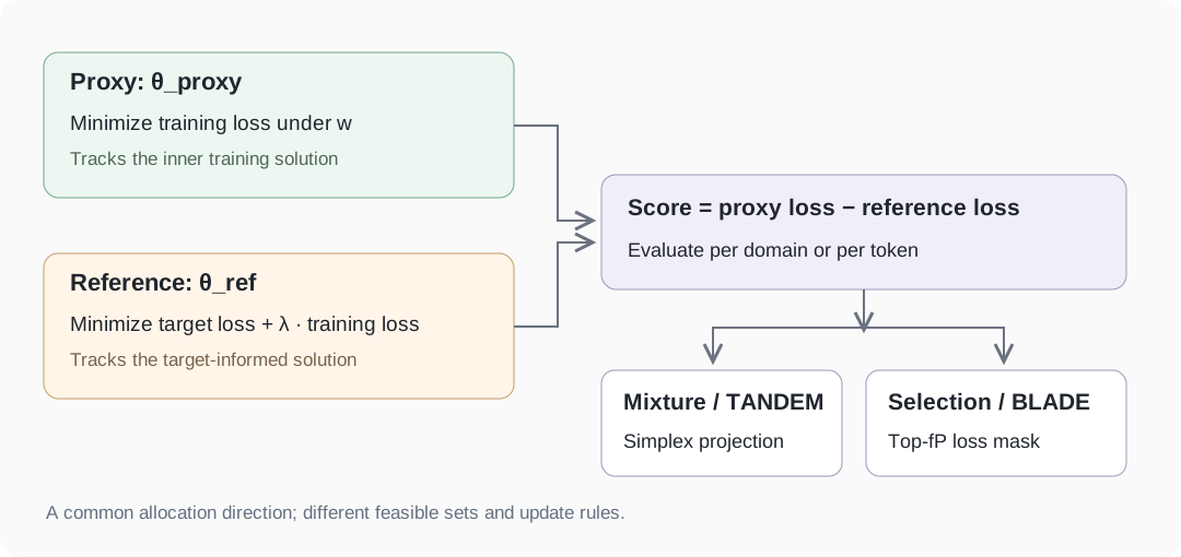
The shared penalty-based solver for mixture and selection. Two coupled models produce a loss-difference update signal; the operator’s constraints determine the resulting allocation rule.

TANDEM: which domains deserve more exposure?

Suppose we can adjust how often the learner sees each of $K$ domains. Here $w_k$ is the probability of sampling domain $k$, and $\mathcal L_{\mathrm{train}}^k(\theta)$ is the model’s expected training loss on that domain. The shared bilevel formulation takes the following concrete form:

Component	TANDEM
Target loss	A weighted average of held-out losses across domains. The target weights $\widehat w_k$ specify each domain’s contribution to evaluation (typically, $\widehat w_k=1/K$). These weights stay fixed while the training proportions $w$ are optimized.
Training loss	$\mathcal L_{\mathrm{train}}(\theta;w)=\sum_{k=1}^K w_k\mathcal L_{\mathrm{train}}^k(\theta)$.
Feasible allocations	Domain proportions on the probability simplex $\mathcal W_{\mathrm{mix}}$: $w_k\geq0$ and $\sum_k w_k=1$.

The training loss shows the linear dependence on $w$ used in the shared solver: each domain weight multiplies its domain loss. Differentiating with respect to $w_k$ therefore returns $\mathcal L_{\mathrm{train}}^k(\theta)$. This is why the shared solver’s difference of training-loss derivatives becomes a difference of domain losses between the reference and proxy, giving the allocation gradient estimate $-\lambda s_k$. A projected-gradient step turns it into a new mixture:

\[w^{(t+1)} =\Pi_{\mathcal W_{\mathrm{mix}}} \left(w^{(t)}+\eta_w\lambda s^{(t)}\right).\]

At the domain level, a larger positive $s_k$ means that incorporating target information has improved predictions on domain $k$: the reference has lower domain loss than the training-only proxy. The update gives such domains upward pressure in the training mixture. Projection keeps the probabilities nonnegative and summing to one. The learned mixture is then used to train a fresh final model.

For a concrete result, consider the data-restricted SlimPajama experiment: a 160M model trained from a 300M-token candidate corpus, with smaller domains repeatedly sampled. TANDEM’s learned mixture reduces averaged perplexity from 31.53 under Uniform to 28.07, under the same final-training protocol. Here averaged perplexity is the exponential of the mean held-out domain loss.

What initially surprised me was how little there was to gain in the data-abundant, single-pass pretraining: TANDEM achieved an averaged perplexity of 25.43, compared with 25.74 under Uniform. In this experiment, both Uniform training and target evaluation assign weight $1/K$ to each domain, and their within-domain data come from the same underlying distributions. The population objectives therefore match. Abundant data allows training without repeated exposure to individual samples, and the observed train–validation gaps remain close to zero. Later, the work discussed in Part 1 helped make sense of this contrast: this matched regime leaves little distributional mismatch for reweighting to correct. The solver was effective, but the task offered limited headroom for advancement.

BLADE: which tokens deserve the budget?

A domain is a blunt unit of intervention. Useful and unhelpful material can occur in the same document, or even the same reasoning trace. We therefore move the allocation decision down to individual tokens. Here $w_p$ indicates whether candidate token $p$ contributes to training: one means retained, zero means masked. $\mathcal L_{\mathrm{train}}^p(\theta)$ is then the prediction loss at token position $p$. For a pool of $P$ candidates, we retain a fraction $f$. The shared bilevel formulation takes the following concrete form:

Component	BLADE
Target loss	Prediction loss on the target validation data, $\mathcal L_{\mathrm{target}}(\theta)$.
Training loss	Average loss over retained token positions: $\mathcal L_{\mathrm{train}}(\theta;w)=\frac{1}{fP}\sum_{p=1}^P w_p\mathcal L_{\mathrm{train}}^p(\theta)$.
Feasible allocations	A token mask with $w_p\in\lbrace 0,1\rbrace$ and $\sum_p w_p=fP$.

The training loss shows the same linear dependence on $w$, so the shared solver gives a token-level loss-difference update, with allocation gradient estimate $-\lambda s_p/(fP)$. To optimize the binary mask, we relax $w_p\in\lbrace 0,1\rbrace$ to $w_p\in[0,1]$, keeping the same budget. The resulting feasible set is a capped simplex.

In TANDEM, domain proportions are continuous probabilities constrained to sum to one, so we use projected gradient descent to keep each update within the simplex. BLADE instead requires a keep-or-discard decision for each token. We temporarily allow fractional token weights to make this discrete problem amenable to continuous optimization. Frank–Wolfe then gives an elegant result: with a full, greedy step, the update lands directly on a binary mask—the $fP$ tokens with the largest loss-difference scores—with no extra rounding needed:

\[w_p =\mathbf 1\left\{p\in\operatorname{Top}_{fP}(s)\right\}.\]

The token-level loss difference reflects the predictive improvement associated with target-informed training, providing a signal for which tokens may help align the learner with the target. To make this criterion practical at corpus scale, BLADE applies the selection rule within candidate batches, enabling online token selection without scoring and storing the entire corpus in advance.

We evaluate token selection by continually pretraining a 13B language model on a 5B-token OpenWebMath pool. Across nine math-related benchmarks, BLADE achieves 54.4% average accuracy, compared with 52.5% for RHO-1 and 43.7% for full-pool continual pretraining. BLADE and RHO-1 each retain 3B loss-bearing tokens, while full-pool training uses all 5B tokens.

TANDEM and BLADE use the same proxy/reference construction to update training exposure. The constraints turn that update into domain proportions in one case and a Top-$k$ token mask in the other. The loss-difference update depends jointly on the target and the learned states of the proxy and reference models. These states reflect the learning procedure and the combined effect of the training examples, including how their learning signals overlap or complement one another. This makes the perspective of Part 2 concrete: the criterion evaluates data through a learner and a target, rather than assigning each domain or token an intrinsic quality score.

Synthesis: when reallocation is not enough

Both data mixture and selection assume useful training material is somewhere in the pool. What if it is not? A curator cannot recover an absent tool-use example, failure-recovery pattern, or reasoning strategy. Synthesis lets us make the examples themselves part of the decision.

As with mixture and selection, synthesis is evaluated by the target performance of the model trained on the resulting data. The distribution-level objective remains the same, but its parameterization changes. Let $\psi$ control a generator, its prompts, or its task specifications, inducing a training distribution $q_\psi$. Writing $\theta^*(\psi)$ for the model trained on $q_\psi$, the problem becomes

\[\min_{\psi\in\Psi} \mathcal L_{\mathrm{target}}\!\left(\theta^*(\psi)\right) \quad\text{s.t.}\quad \theta^*(\psi)\in\arg\min_\theta \mathbb E_{x\sim q_\psi}[\ell(x;\theta)].\]

The permitted generation parameters $\Psi$ and the generation budget define the reachable family $\mathcal Q_{\mathrm{synth}}={q_\psi:\psi\in\Psi}$. Generation can introduce missing modes or add examples within existing ones.

For mixture and selection, the training loss depends linearly on the allocation weights, yielding a simple loss-difference update. Whether an equally simple and efficient update can be obtained when the decision changes the generated examples themselves remains an open question for extending this solver to synthesis.

These operators, mixture, selection and synthesis, can also work together in a target-driven data pipeline. One practical loop I use is:

Target failures → identify missing training material → generate candidates → select or verify → train the model → evaluate on the target.

In this loop, an LLM generates candidates and target-guided selection determines what to retain, bypassing the need to solve the bilevel generation problem.

Target, Gap and operator

Across these three essays, the questions have moved from what kind of improvement we obtained, to what makes a training distribution valuable, to how we can change it in practice.

For a new data problem, the starting questions are what target matters, where ordinary training falls short, and whether the available data contains material that can help. These answers guide the choice of operator and how to optimize it.

Or, in three lines:

Target defines the objective.
Gap defines the headroom.
Operator defines the reachable improvement.

Data design begins when those three are specified together.