The 3.5-Point Win That Disappeared: Advancement vs. Acceleration
Designing Training Data for Language Models · Part 1 of 3
When to optimize, what makes data good, and how to change it.
Advancement vs. Acceleration · What Makes Data Good? · From Target to Operator
We had been trying to improve a language model’s capability by optimizing its training-data mixture. The hope was simple: if we allocated the token budget more intelligently across domains, perhaps the resulting model would become genuinely better.
For one experiment, following the setup from Aioli, we search for the optimal data mixture on seven SlimPajama domains—ArXiv, Books, C4, CommonCrawl, GitHub, StackExchange, and Wikipedia. We tried RegMix, which trains small proxy models on different mixtures, fits a regression model to their outcomes, and uses it to propose a promising mixture for a larger run. A fresh model is trained under that RegMix-optimized mixture after the optimal mixture is obtained.
At 2,000 training steps, this new model beat the one trained with a uniform mixture by 3.5 averaged-perplexity points. It looked like exactly the result we had hoped for. If we had stopped there—as fixed-budget comparisons often do—we would have called it a convincing success.
Then we kept the same run going, consuming more training data.
The gap shrank. And shrank. By the end, it was gone.
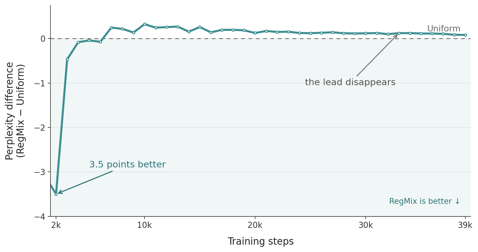
RegMix is 3.5 perplexity points better at 2,000 steps. At the final checkpoint it is slightly worse than Uniform: the important observation is not that the two runs become identical, but that RegMix no longer retains an advantage.
That disappearing win left me with a question that eventually became the focus of this work:
When data curation improves a language model, does it change what the model can ultimately learn, or only how quickly it gets there?
The result was real, but its meaning was narrower than the early checkpoint suggested. RegMix reached a given performance sooner without producing a better attainable model.
This is where I find a lot of discussion around data curation surprisingly slippery. We use the word improvement for two different things:
Acceleration changes how quickly we reach a level of performance.
Advancement changes the best level of performance we can eventually reach.
Acceleration can be valuable in its own right: reaching the same capability with substantially fewer tokens is a meaningful gain. Here, though, I am interested in a different question: can changing the training data improve the attainable endpoint? The disappearing advantage in our experiment made that distinction worth examining.
The endpoint and the road to it
Let $\mathcal E_\alpha(w)$ denote target performance after training with data budget $\alpha$ under curation policy $w$. The policy may represent domain-mixture weights, example-selection decisions, or token-level masks. To keep the inequalities concrete, write $\mathcal E$ in a lower-is-better orientation—loss, error, or negative accuracy. For an accuracy metric, simply reverse the inequalities.
The endpoint is
\[\mathcal E_\infty(w)=\lim_{\alpha\rightarrow\infty}\mathcal E_\alpha(w).\]A policy provides advancement if
\[\mathcal E_\infty(w)<\mathcal E_\infty(w_0),\]where $w_0$ indicates the uncurated baseline.
For a target performance level $\varepsilon$, let $\alpha_w(\varepsilon)$ be the smallest budget needed to reach it. The policy provides acceleration if
\[\alpha_w(\varepsilon)<\alpha_{w_0}(\varepsilon).\]Acceleration changes the road: the same performance is reached with less data. Advancement changes the destination: the endpoint itself improves. A single checkpoint cannot distinguish the two.
Why would a data method change the endpoint at all?
Suppose I give you a gigantic jar containing red and blue marbles and ask you to reproduce the same red–blue ratio in another jar. A clever sampling strategy may help you estimate the ratio faster. But if ordinary sampling already targets the right distribution, no reweighting trick should produce a more correct answer in the limit.
Data curation has the same basic constraint. Write it as a bilevel problem:
\[\min_w \; \mathcal L_{\mathrm{target}}\!\left(\theta^*(w)\right) \quad\text{s.t.}\quad \theta^*(w)\in\arg\min_\theta \mathcal L_{\mathrm{train}}(\theta;w).\]The inner problem optimizes the model parameters $\theta$. The outer problem optimizes the data policy $w$, which determines the trained model $\theta^(w)$. But if the uncurated training objective already *matches the target objective, where could a better endpoint come from?
The one-line obstruction
Let $w_0$ denote the uncurated baseline and suppose, crucially, that there is no train–target gap at the population level:
\[\mathcal L_{\mathrm{train}}^{\mathrm{pop}}(\theta;w_0) = \mathcal L_{\mathrm{target}}^{\mathrm{pop}}(\theta) \qquad \text{for every }\theta.\]“Matches” means that, under the baseline policy $w_0$, training and target losses are the same function of $\theta$—not just equal at one checkpoint. These are population losses: expectations over the underlying data distributions. In the idealized large-data limit $\alpha\to\infty$, converged training minimizes this objective.
When the inner optimization converges, the baseline solution
\[\theta^*(w_0)\in\arg\min_\theta \mathcal L_{\mathrm{train}}^{\mathrm{pop}}(\theta;w_0)\]also globally minimizes the target objective—because, under $w_0$, the training and target losses are the same function. For any alternative curation policy $w$, its trained solution $\theta^*(w)$ is still another model in the same hypothesis class. Therefore
\[\mathcal L_{\mathrm{target}}^{\mathrm{pop}}\!\left(\theta^*(w_0)\right) = \min_\theta \mathcal L_{\mathrm{target}}^{\mathrm{pop}}(\theta) \leq \mathcal L_{\mathrm{target}}^{\mathrm{pop}}\!\left(\theta^*(w)\right).\]That is the obstruction: when the uncurated baseline already optimizes the target population objective, no reallocation can produce a strictly better target endpoint. This conclusion assumes a fixed model class and converged inner optimization.
The argument is simple, but its implication is easy to overlook in practice. When a better mixture or subset wins at a finite training budget, it is tempting to read that gain as evidence of a better endpoint. Yet without a correctable population gap, the gain can be acceleration alone.
A mixture example. For $K$ domains, let $w_k$ be domain $k$’s training proportion and $\widehat w_k$ its fixed importance in the target. Both weight vectors are nonnegative and sum to one. The population objectives are
\[\begin{aligned} &\mathcal L_{\mathrm{train}}^{\mathrm{pop}}(\theta;w) =\sum_{k=1}^K w_k\mathcal L_{\mathrm{train}}^{k,\mathrm{pop}}(\theta),\\ &\mathcal L_{\mathrm{target}}^{\mathrm{pop}}(\theta) =\sum_{k=1}^K\widehat w_k\mathcal L_{\mathrm{target}}^{k,\mathrm{pop}}(\theta). \end{aligned}\]The training proportions $w$ are the decision. If training and target share the same distribution within each domain and $w_0=\widehat w$, their population objectives are identical—the no-gap condition above.
This is the population picture behind abundant, single-pass training when training and evaluation data are sampled i.i.d. from the same underlying distribution: more data makes the empirical objectives approach the same expected loss.
The seven-domain SlimPajama experiment above uses equal target weights, $\widehat w_k=1/K=1/7$. Its uniform baseline therefore has $w_{0,k}=\widehat w_k$. When training and evaluation sample the same underlying distribution within each domain, this baseline already minimizes the target objective at the population endpoint. The early gains in those learning curves are therefore consistent with acceleration. This remains true even when some domains are harder to learn than others. Giving harder domains more weight may help at finite budgets, but difficulty differences alone do not create room for a better endpoint when the baseline already matches the target.
These results are developed in our forthcoming paper, Advancement or Acceleration? How Data Curation Improves LLM Training.
Lasting advancement requires a correctable train–target gap.
A train–target gap leaves room for advancement, but does not guarantee it. The available data and the way we can change its use must allow us to reduce that gap. This is what correctable means here.
Seeing acceleration and advancement
To make the distinction concrete, we use teacher–student perceptron models: a teacher generates labels, and a student learns from the curated data (see Loureiro et al., 2021 for learning-curve analysis and Sorscher et al., 2022 for data pruning). These models let us study both learning at finite data budgets and the $\alpha\to\infty$ endpoint, distinguishing gains that fade from those that persist. The technical derivations are given in the paper.
Read the figure by rows: mixture above, selection below. The left column shows the setup, the middle shows acceleration without a gap, and the right shows what changes when a gap is present. Here $\alpha=P/N$ measures the data budget in samples per parameter.
Mixture: reweighting can accelerate learning without a gap—and improve the endpoint when it corrects one. To illustrate acceleration, we make domain 2 harder to learn than domain 1 in the top row (see the paper for the construction). The training proportion of domain 1 is $w_1$ and its target weight is $\widehat w_1=0.5$. When $w_1 = \widehat w_1=0.5$(no gap), giving the harder domain more training data helps at small budgets, but the advantage disappears as the budget grows (b). When the target weights change, the best mixture changes with them: panel (c) shows that target matching is optimal at a large but finite budget. In the paper, we further show that this optimality holds as $\alpha\to\infty$, even when domain difficulty differs.
Selection: pruning can accelerate learning without a gap—and improve the endpoint when it corrects one. In the bottom row, we construct the training and target labeling rules using two linear perceptron teachers. Each is described by a vector normal to its decision boundary: $B$ for training and $B_{\mathrm{tar}}$ for the target. The angle $\phi$ between them controls the train–target mismatch (d). The retained fraction is $f$, so $f=1$ means keeping everything. We select examples using a criterion that favors those near the target decision boundary and penalizes those whose training labels disagree with the target teacher. Without a gap, moderate pruning can preserve accuracy with less data, but cannot improve the endpoint (e). With a gap, selection trades off fewer training examples against better alignment with the target. Panel (f) shows that the alignment benefit can outweigh the loss of data. In the paper, we show that the gain can persist as $\alpha\to\infty$.
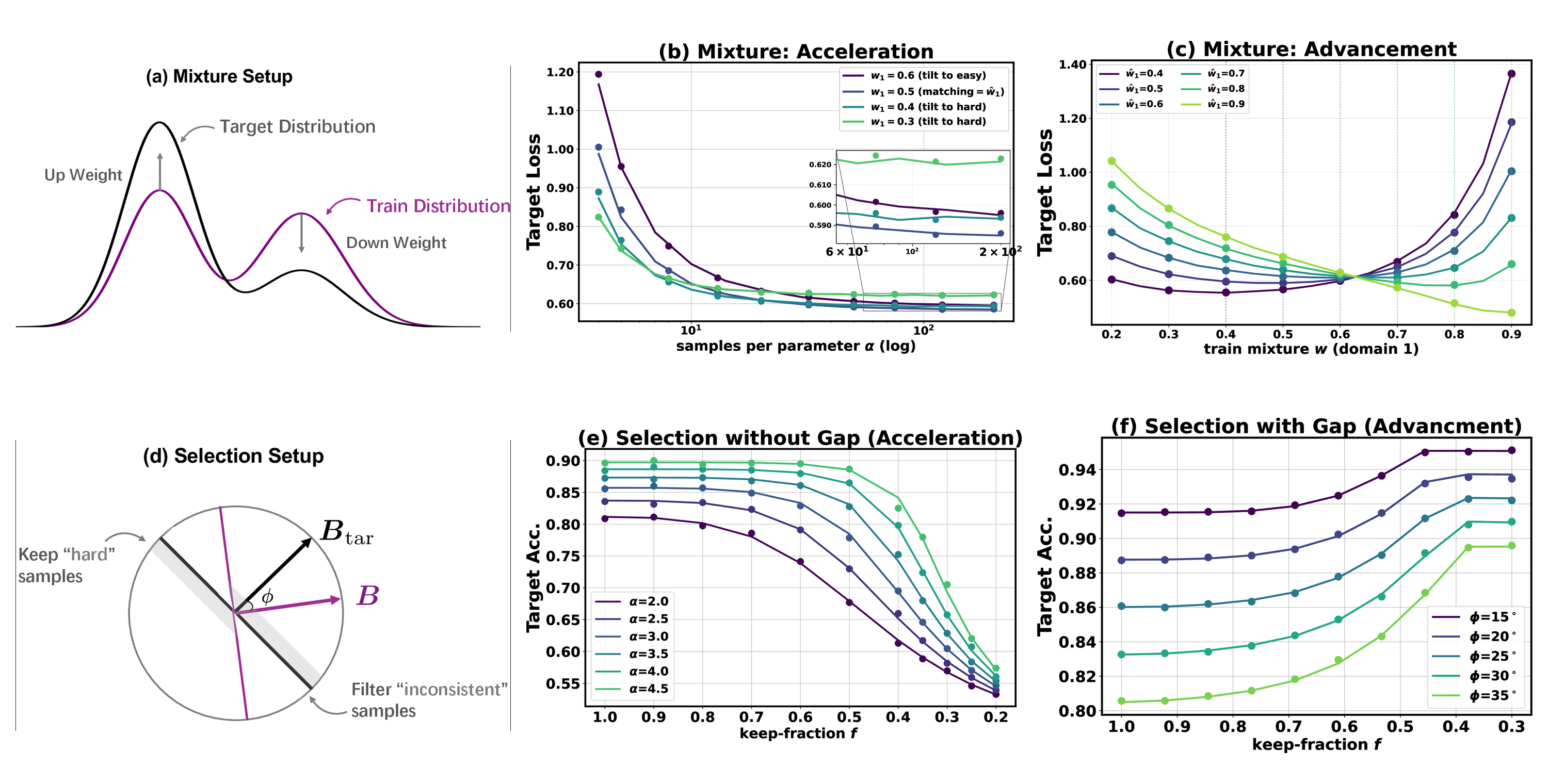
In the top row, lower target loss is better. In the bottom row, higher target accuracy is better. The selection plots run from full retention on the left to stronger pruning on the right. Solid lines are theoretical predictions and circles are simulations with $N=200$.
A one-run diagnostic before an expensive search
The population condition is clean but cannot usually be checked directly on real corpora. We therefore use the $\Delta$-test as an observable diagnostic from an ordinary uncurated baseline run. Let $\theta$ denote a model checkpoint from that run; the diagnostic does not require training to have converged.
For a $K$-domain mixture,
\[\Delta = \sum_{k=1}^{K} \left| \widehat w_k\mathcal L_{\mathrm{target}}^k\!\left(\theta\right) - w_{0,k}\mathcal L_{\mathrm{train}}^k\!\left(\theta\right) \right|.\]Here $\widehat w_k$ is domain $k$’s importance in the target distribution, while $w_{0,k}$ is its exposure under the uncurated training mixture.
For selection, there is a single candidate pool, so the diagnostic reduces to
\[\Delta = \left| \mathcal L_{\mathrm{target}}\!\left(\theta\right) - \mathcal L_{\mathrm{train}}\!\left(\theta\right) \right|,\]where $w_0$ means full retention.
In our experiments, the $\Delta$-test provides a useful early signal: appreciably nonzero values indicate opportunities for persistent gains, while gains near $\Delta=0$ tend to fade as the budget grows. A near-zero $\Delta$ suggests limited headroom, though it does not rule out every train–target gap. Note that $\Delta$ is not a sufficient condition for advancement: the available data and policy still determine whether the detected gap can be corrected.
Controlled interventions on the gap
We tested two questions in both mixture and selection experiments: do curation gains depend on the train–target gap, and can the $\Delta$-test identify promising tasks before an expensive search? We varied the train–target gap while keeping the methods and training setup largely unchanged.
The experiments below track gains within the training budgets we tested; the infinite-data conclusions come from the analysis above. The reported $\Delta$ values are measured halfway through the uncurated baseline’s training budget, rather than after full convergence. In practice, we can use a small proxy model for diagnosis before larger runs to reduce additional computation.
For mixture, we compared Uniform with Skill-It, RegMix, Aioli, DoGE, and TANDEM:
- Matched regime ($\Delta=0.07$). This is the seven-domain SlimPajama setting from the opening experiment. Training and target weight the domains equally, and the pool is large enough to avoid repeatedly sampling depleted domains. Final averaged perplexities ranged from 19.66 to 20.17, statistically close to Uniform at 19.71. By the final checkpoint, the early leads had disappeared within experimental variation.
- Endogenous gap ($\Delta=0.64$). We keep the same uniformly weighted target but restrict the pool to 300M tokens, preserving its original domain proportions. Small domains such as ArXiv and Wikipedia run out early and are repeatedly sampled. Overfitting lowers their training losses relative to held-out target losses: the gap is endogenous because it develops through training on limited data. Optimized mixtures improve performance by reducing exposure to these overfit domains.
- Exogenous gap ($\Delta=1.26$). We hold out CommonCrawl as the target and train on the remaining six domains. The gap is exogenous because the target distribution differs from the candidate training pool. Related data such as C4 still offers a way to partially correct the mismatch by reweighting. Target perplexity fell from 49.19 under Uniform to roughly 40–41 under optimized mixtures.
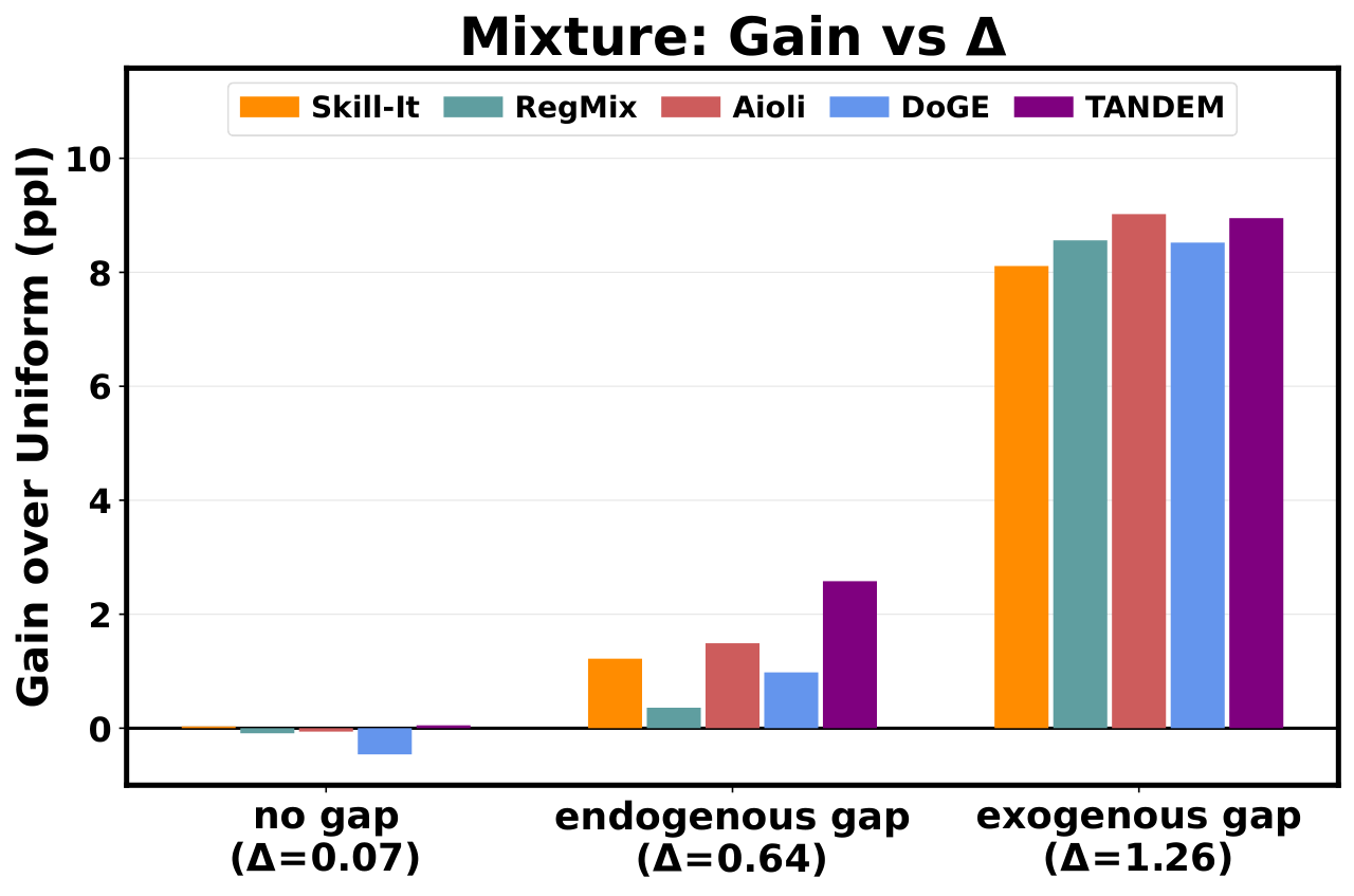
The same mixture methods produce negligible gains by the final checkpoint in the approximately matched regime, while gains remain through the largest tested budget in settings with correctable gaps.
Selection provides a paired control. We kept the model, 5B-token OpenWebMath candidate pool, 60% keep ratio, and training protocol fixed. We compared Random, EL2N, InfoBatch, Token-Cleaning, RHO-1, and BLADE, alongside full-pool continual training. Using the same methods in both settings, we changed only the target used for selection and evaluation.
- With an in-distribution OpenWebMath target, $\Delta=0.016$ and no selector consistently beat full-pool continual training.
- With a shifted MetaMath–MAmmoTH target, $\Delta=0.549$. Target-aware RHO-1 and BLADE could now correct a visible mismatch. BLADE raised average benchmark accuracy from 17.21 to 31.31 while retaining 60% of the candidate tokens.
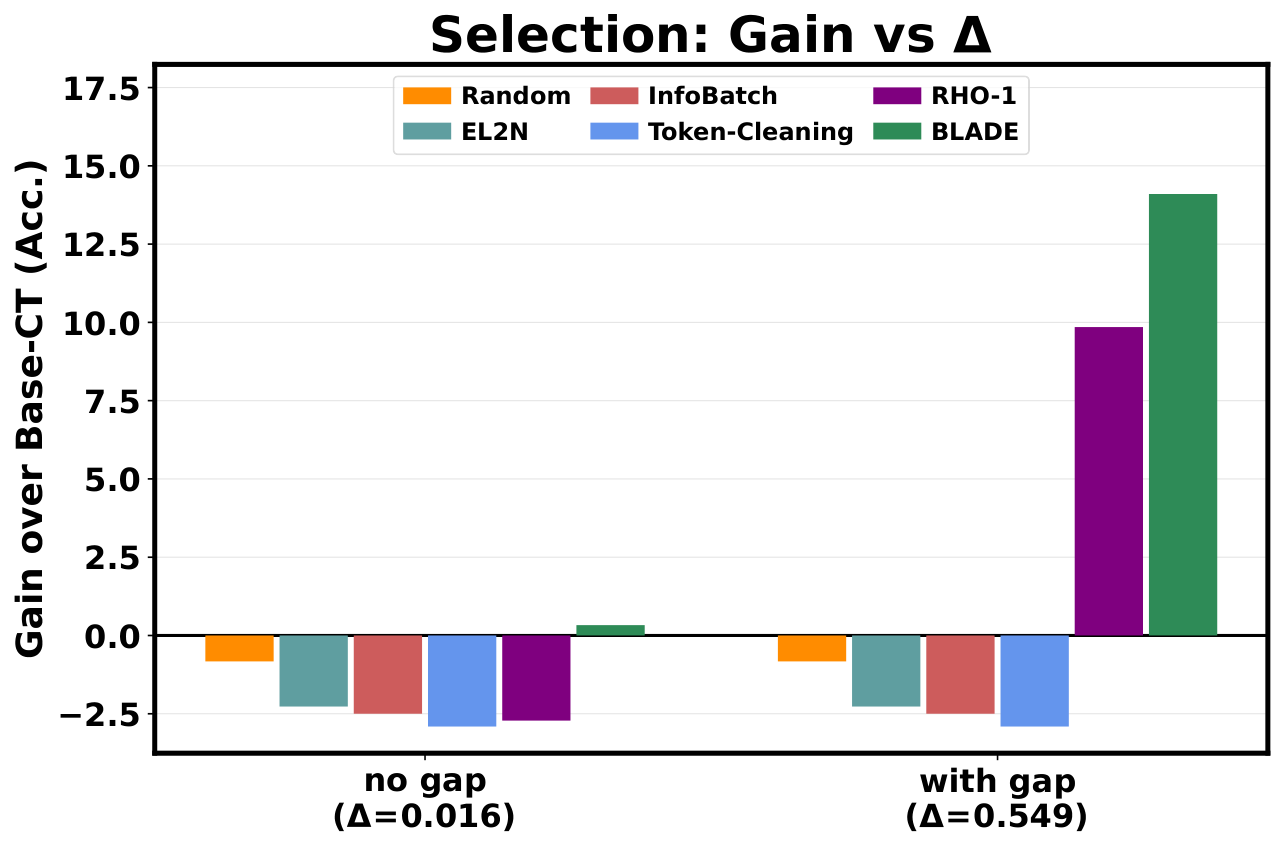
Selection yields little improvement over full-pool continual training in the approximately matched setting, but substantial gains with a correctable gap. The $\Delta$-test distinguishes these settings before selection.
A different order of operations
These results suggest that before asking which curation method to use, we should ask what improvement the task leaves room for. The $\Delta$-test offers a practical starting point for that diagnosis.
A common data curation workflow begins with the method:
- Invent a data-utility scoring rule.
- Select or reweight data.
- Train a model.
- Hope the target metric improves.
I would instead start with the task:
- Define the target. What distribution and metrics represent the capability we actually care about?
- Run the uncurated reference and diagnose the task. Estimate $\Delta$ with a small proxy when possible.
- Check correctability. Does the candidate pool contain the missing modes, and can mixture or selection expose them?
- Specify the claim and optimize the data. Are we trying to save compute, move the attainable endpoint, or both?
- Validate accordingly. For acceleration, report tokens, FLOPs, or wall-clock time at matched performance. For advancement, increase the budget and test whether the advantage persists.
Reaching the same capability with less compute and improving the attainable endpoint are both useful. They answer different questions and call for different evaluations. In either case, the value of changing the data depends on the target. This raises a further question: can training data be called “high quality” before we specify what we want the learner to achieve?
That is the subject of the next essay.